
data-mining-distribution
Foreword
这里介绍数据挖掘中如何对数据进行分布检测。
示例数据iris
import os
import random

import pandas as pd
import numpy as np

import statsmodels.api as sm
import statsmodels.stats.multicomp
from statsmodels.formula.api import ols
from statsmodels.stats.anova import anova_lm

from matplotlib import pyplot

from sklearn.datasets import load_iris
from sklearn.model_selection import train_test_split

from scipy import stats

import seaborn as sns
# 设置matplotlib默认属性
sns.set_context("paper", font_scale=1.3)
# 设置主题:
# darkgrid 黑色网格(默认)
# whitegrid 白色网格
# dark 黑色背景
# white 白色背景
# ticks 四周都有刻度线的白背景
sns.set_style('white')

# 统计假设检验阈值
alpha = 0.05

# 以iris数据集为例
iris = load_iris()
X = iris['data']
y = iris['target']

X_train, X_test, y_train, y_test = train_test_split(X, y, train_size=0.7)

# 取特征数据进行分析
feature_0 = X[:, 0]
feature_1 = X[:, 1]
feature_2 = X[:, 2]
feature_3 = X[:, 3]
绘图查看
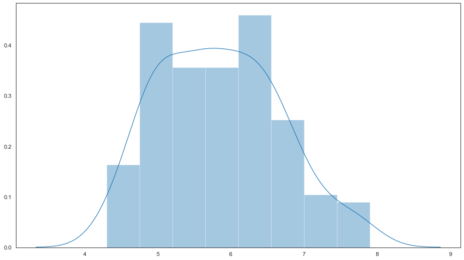
绘制直方图并拟合内核密度估计
绘制直方图并拟合内核密度估计。通过调整参数可以分别绘制直方图,拟合内核密度图,地毯图等。查看直方图分布,能更好的可视化特征数据分布。
fig, ax = pyplot.subplots(figsize=(16, 9))

# 绘制直方图并拟合内核密度估计
sns.distplot(feature_0, ax=ax)
<matplotlib.axes._subplots.AxesSubplot at 0x7ff9d1563b10>
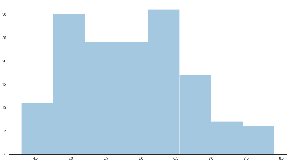
绘制直方图
当绘制直方图时,需要调整的参数是bin的数目(组数)。displot()会默认给出一个它认为比较好的组数,尝试不同的组数可能会揭示出数据不同的特征。
# 绘制直方图
fig, ax = pyplot.subplots(figsize=(16, 9))

sns.distplot(feature_0, ax=ax, kde=False)
<matplotlib.axes._subplots.AxesSubplot at 0x7ff9cce85650>
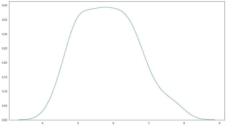
绘制核密度估计图
核密度估计图使用的较少,但其是绘制出数据分布的有用工具,与直方图类似,KDE图以一个轴的高度为准,沿着另外的轴线编码观测密度。
# 绘制核密度估计图
fig, ax = pyplot.subplots(figsize=(16, 9))

sns.distplot(feature_0, ax=ax, hist=False)
<matplotlib.axes._subplots.AxesSubplot at 0x7ff9d23695d0>
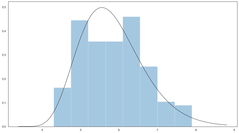
绘制拟合参数分布图
拟合出一个数据集的参数分布,直观上来评估其余观测数据是否关系密切。
# 绘制拟合参数分布图
fig, ax = pyplot.subplots(figsize=(16, 9))

sns.distplot(feature_0, ax=ax, kde=False, fit=stats.gamma)
<matplotlib.axes._subplots.AxesSubplot at 0x7ff9d2814b10>
统计分布
偏度检测
偏度(Skewness)检测确定数据分布是否偏离正态分布,测试数据度量分布的不对称性:
计算方式为随机变量的三阶标准中心矩为:
\[\operatorname{Skewness}[X]=\mathrm{E}\left[\left(\frac{X-\mu}{\sigma}\right)^{3}\right]=\frac{\mathrm{E}\left[(X-\mu)^{3}\right]}{\left(\mathrm{E}\left[(X-\mu)^{2}\right]\right)^{3 / 2}}=\frac{\mu_{3}}{\sigma^{3}}\]如果偏度介于 -0.5 和 0.5 之间,则数据是基本对称的。
如果偏度介于 -1 和 -0.5 之间或者 0.5 和 1 之间,则数据是稍微偏斜的。
如果偏度小于 -1 或大于 1, 则数据是高度偏斜的。
数据量分布:
正态分布的偏度为0,则:两侧尾部长度对称;
偏度为负,即负偏离(左偏离),则:数据位于平均值左边的比右边的少,直观表现为左边的尾部相对于右边的尾部要长。
偏度为正,即正偏离(右偏态),则:数据位于平均值右边的比左边的少,直观表现为右边的尾部相对于左边的尾部要长。
平均数、中位数、众数关系:
右偏时:平均数>中位数>众数
左偏时:众数>中位数>平均数
正态分布三者相等
# 偏度检测
print('Skewness of normal distribution: {}'.format(stats.skew(feature_0)))
Skewness of normal distribution: 0.3117530585022963
峰度检测
峰度用于描述特征数据分布的尾重:
计算方式为随机变量的四阶标准中心矩: \(\operatorname{Kurt}[X]=\mathrm{E}\left[\left(\frac{X-\mu}{\sigma}\right)^{4}\right]=\frac{\mathrm{E}\left[(X-\mu)^{4}\right]}{\left(\mathrm{E}\left[(X-\mu)^{2}\right]\right)^{2}}=\frac{\mu_{4}}{\sigma^{4}}\)
正态分布的峰度接近于 0。如果峰度大于 0,则分布尾部较重。
如果峰度小于 0,则分布尾部较轻。
# 峰度检测
print('Kurtosis of normal distribution: {}'.format(stats.kurtosis(feature_0)))
Kurtosis of normal distribution: -0.5735679489249765
统计正态性检验
正态性检验量化数据是否符合高斯分布,p值做出如下解释:
H0,原假设;H1,备则假设。p值越小越能否定H0。
p <= alpha:拒绝 H0,非正态。
p > alpha:不拒绝 H0,正态。
Shapiro-Wilk试验
w, p = stats.shapiro(feature_0)
print("w=%0.4f, p=%.4f"% (w, p))

if p < alpha:  # null hypothesis: x comes from a normal distribution
    print("The null hypothesis can be rejected")
else:
    print("The null hypothesis can not be rejected")
w=0.9761, p=0.0102
The null hypothesis can be rejected
Q-Q图试验
fig = sm.qqplot(feature_0, line='s')
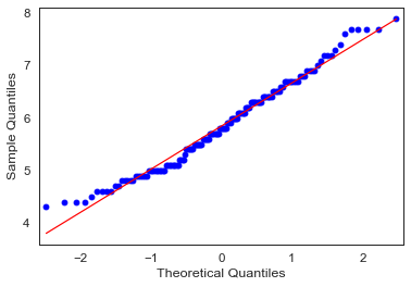
从上图中,看到所有数据点都靠近 y=x,因此我们可以得出结论,它遵循正态分布。
#### 统计正态性检验
s2k2, p = stats.normaltest(feature_0)
print('s2k2=%.3f, p=%.3f' % (s2k2, p))

if p < alpha:  # null hypothesis: x comes from a normal distribution
    print("The null hypothesis can be rejected")
else:
    print("The null hypothesis can not be rejected")
s2k2=5.736, p=0.057
The null hypothesis can not be rejected
ANOVA方差分析
方差分析,可以看作是两组以上的t检验的推广。独立t检验用于比较两组之间的条件平均值。当我们想比较两组以上特征数据平均值时,使用方差分析。 方差分析测试模型中某个地方的平均值是否存在差异(测试是否存在整体效应),但它不能告诉我们差异在哪里(如果存在)。为了找出两组之间的区别,我们必须进行事后检验。 要执行任何测试,我们首先需要定义原假设和替代假设:
零假设–各组之间无显着差异
替代假设–各组之间存在显着差异
基本上,方差分析是通过比较两种类型的变化来完成的,即样本均值之间的变化,以及每个样本内部的变化。
### 单因素方差分析
F, p = stats.f_oneway(feature_0, feature_1, feature_2, feature_3)

alpha = 0.05

## 看看整体模型是否重要
print('F-Statistic=%.3f, p=%.3f' % (F, p))

if p < alpha:  # null hypothesis: 零假设–各组之间无显着差异
    print("The null hypothesis can be rejected")
else:
    print("The null hypothesis can not be rejected")
F-Statistic=482.915, p=0.000
The null hypothesis can be rejected
事后比较检验
当我们进行方差分析时,我们试图确定各组之间是否存在统计学上的显着差异。那么,如果我们发现统计学意义呢?
如果发现存在差异,则需要检查组差异的位置。因此,我们将使用Tukey HSD测试来确定差异所在:
mc = statsmodels.stats.multicomp.MultiComparison(feature_0[0:9],
                                                 feature_1[0:9])
mc_results = mc.tukeyhsd()
print(mc_results)
Multiple Comparison of Means - Tukey HSD, FWER=0.05
====================================================
group1 group2 meandiff p-adj  lower    upper  reject
----------------------------------------------------
   2.9    3.0      0.5   0.1 -12.3364 13.3364  False
   2.9    3.1      0.2   0.1 -12.6364 13.0364  False
   2.9    3.2      0.3   0.1 -12.5364 13.1364  False
   2.9    3.4      0.4   0.1 -10.7166 11.5166  False
   2.9    3.5      0.7   0.1 -12.1364 13.5364  False
   2.9    3.6      0.6   0.1 -12.2364 13.4364  False
   2.9    3.9      1.0   0.1 -11.8364 13.8364  False
   3.0    3.1     -0.3   0.1 -13.1364 12.5364  False
   3.0    3.2     -0.2   0.1 -13.0364 12.6364  False
   3.0    3.4     -0.1   0.1 -11.2166 11.0166  False
   3.0    3.5      0.2   0.1 -12.6364 13.0364  False
   3.0    3.6      0.1   0.1 -12.7364 12.9364  False
   3.0    3.9      0.5   0.1 -12.3364 13.3364  False
   3.1    3.2      0.1   0.1 -12.7364 12.9364  False
   3.1    3.4      0.2   0.1 -10.9166 11.3166  False
   3.1    3.5      0.5   0.1 -12.3364 13.3364  False
   3.1    3.6      0.4   0.1 -12.4364 13.2364  False
   3.1    3.9      0.8   0.1 -12.0364 13.6364  False
   3.2    3.4      0.1   0.1 -11.0166 11.2166  False
   3.2    3.5      0.4   0.1 -12.4364 13.2364  False
   3.2    3.6      0.3   0.1 -12.5364 13.1364  False
   3.2    3.9      0.7   0.1 -12.1364 13.5364  False
   3.4    3.5      0.3   0.1 -10.8166 11.4166  False
   3.4    3.6      0.2   0.1 -10.9166 11.3166  False
   3.4    3.9      0.6   0.1 -10.5166 11.7166  False
   3.5    3.6     -0.1   0.1 -12.9364 12.7364  False
   3.5    3.9      0.3   0.1 -12.5364 13.1364  False
   3.6    3.9      0.4   0.1 -12.4364 13.2364  False
----------------------------------------------------
Tuckey HSD测试清楚地表明,feature_0和feature_1前10个样本之间存在显着差异(显然的,用的不同特征的数据)。
处理非正态分布数据
前面介绍检测数据分布的方法,那当发现数据不符合预设分布时候,该如何处理呢?我们可以使用Box-Cox转换将数据转换为正态分布。
具体转换方法,请查看:标准化-非线性变换-映射到高斯分布
Reference
更多内容,请参考以下链接:
https://juejin.im/post/5ee8c79a6fb9a047ed242091
https://blog.shinelee.me/2020/07-08-%E6%8D%9F%E5%A4%B1%E5%87%BD%E6%95%B0%E6%98%AF%E5%AD%A6%E4%B9%A0%E7%9A%84%E6%8C%87%E6%8C%87%E6%8C%A5%E6%A3%92%E2%80%94%E8%AE%B0%E4%B8%80%E6%AC%A1%E5%B7%A5%E4%BD%9C%E5%AE%9E%E8%B7%B5.html
Comments powered by Disqus.